SAR11pres05

SAR11 Bacteria Comparative Genomics Project

SAR11 is a group of small, carbon-oxidizing bacteria that reach a global estimated population size of 2.4×10²⁸ cells-approximately 25% of all plankton. They play a key role in the ocean’s environment.

The goal of this comparative genomics project is to find presense and absence of SAR11 genomes. The genomes of interest were obtained from NCBI database.

Methods

• Determine goal of the project
• Decided which genomes to use and obtained them from the NCBI database
• Coding
  • Make a database
  • Get the query sequence
  • Run BLAST
  • Joining blast table with annotation table

The code was based on week 01 assignment from Fish546 Spring 23.

Code 1.1

Created two plots and one table.

In the following slides there will be:

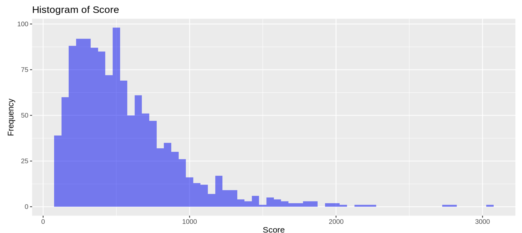
• Histogram for the Scoring for the comparing of two genomes

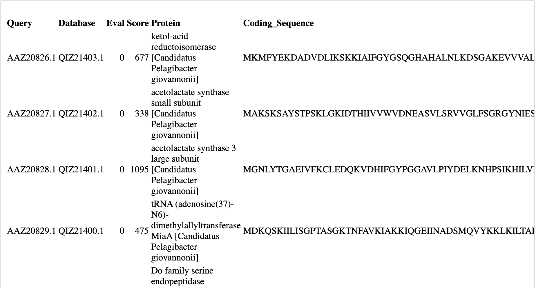
• Table of the joined annotation table and BLAST

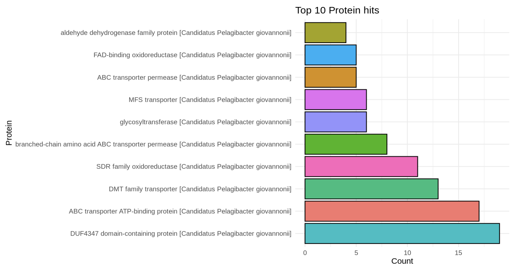
• Bar plot of the top 10 protein hits

Initial Code

/home/shared/ncbi-blast-2.11.0+/bin/makeblastdb \
-in ../data_raw/012276695protein.faa \
-dbtype prot \
-out ../blastdb/95-protein

/home/shared/ncbi-blast-2.11.0+/bin/blastp \
-query ../data_raw/000012345.1protein.faa \
-db ../blastdb/95-protein \
-out ../output/95-45_blastp.tab \
-evalue 1E-20 \
-num_threads 20 \
-max_target_seqs 1 \
-outfmt 6

Histogram for the BLAST file of 95-45

# Read FASTA file

blast_file <- read.csv("../output/95-45_blastp.tab", sep = '\t', header = FALSE) 

#Extract columns desired

blast2.0_file <- blast_file[, c("V1", "V2", "V11", "V12")]

#Make into dataframe

blast2.0_file_df <- data_frame(blast2.0_file)
colnames(blast2.0_file_df) <- c("Query", "Database", "Eval", "Score")

# Plot histogram using ggplot2

ggplot(blast2.0_file_df, aes(x = Score)) +
  geom_histogram(binwidth = 50, fill = "blue", alpha = 0.5) +
  labs(title = "Histogram of Score", x = "Score", y = "Frequency")

Histogram Figure

Table for the combination of BLAST of 95-45

#Having the comparison of 95 to 45 into a CSV file.

# Read out the blast file into csv
bltabl <- read.csv("../output/95-45_blastp.tab", sep = '\t', header = FALSE)


#Extract columns desired
 bltabl_2.0 <- bltabl[, c("V1", "V2", "V11", "V12")]

#Make into dataframe

bltabl2.0_df <- data_frame(bltabl_2.0)

colnames(bltabl2.0_df) <- c("Query", "Database", "Eval", "Score")

#Reading the file from 95 protein to CSV file.

spgo <- read.csv("../output/95protein.tab", sep = '\t', header = TRUE)
colnames(spgo) <- c("Database", "Protein", "Coding_Sequence")

# Join the data frames
joined_df <- left_join(bltabl2.0_df, spgo, by = c("Database" = "Database"))

# Print the table with kable
kable(head(joined_df, n = 10), caption = "Joined data frame with kable formatting (first 10 rows)") 

Table Figure

Plotting the top 10 Protein Hits

# Read joined blast table with annotation table
joined_df <- left_join(bltabl2.0_df, spgo, by = c("Database" = "Database"))

# Select the column of interest
column_name <- "Protein"  # Replace with the name of the column of interest
column_data <- joined_df[[column_name]]

# Count the occurrences of the strings in the column
string_counts <- table(column_data)

# Convert to a data frame, sort by count, and select the top 10
string_counts_df <- as.data.frame(string_counts)
colnames(string_counts_df) <- c("String", "Count")
string_counts_df <- string_counts_df[order(string_counts_df$Count, decreasing = TRUE), ]
top_10_strings <- head(string_counts_df, n = 10)

# Plot the top 10 most common strings using ggplot2
ggplot(top_10_strings, aes(x = reorder(String, -Count), y = Count, fill = String)) +
  geom_bar(stat = "identity", position = "dodge", color = "black") +
  labs(title = "Top 10 Protein hits",
       x = column_name,
       y = "Count") +
  theme_minimal() +
  theme(legend.position = "none") +
  coord_flip()

Barplot Figure

Next Steps:

• fasta to tab-delimited for the protein sequences to finish the joining
• figure out how this process can be done for multiple protein sequences from other SAR11 sequences
  • which sequences to be chosen?
• tyding up the figures that come from other pieces of code (understanding what the code does)