02-Apul-reference-annotation
================
Kathleen Durkin
2024-08-20
- 1 Genome
- 1.1 Retrieve genome fasta
file
- 1.2
Database Creation
- 1.2.1 Obtain Fasta
(UniProt/Swiss-Prot)
- 1.2.2 Making the database
- 1.3 Running
Blastx
- 1.4 Joining Blast table
with annoations.
- 1.4.1 Prepping Blast
table for easy join
- 1.4.2
Could do some cool stuff in R here reading in table
- 2 Transcriptome
- 2.1 Retrieve transcriptome
fasta file
- 2.2
Database Creation
- 2.2.1 Obtain Fasta
(UniProt/Swiss-Prot)
- 2.2.2 Making the database
- 2.3 Running
Blastx
- 2.4 Joining Blast table
with annoations.
- 2.4.1 Prepping Blast
table for easy join
- 2.4.2
Could do some cool stuff in R here reading in table
Code to annotate our *A. pulchra* reference files (the *A. pulchra*
genome) with GO information
# 1 Genome
## 1.1 Retrieve genome fasta file
We’re using a new A.pulchra genome file annotated by collaborators,
which has not been yet been formally published. (stored locally at
`../data/Apulchra-genome.fa`, `../data/Apulcra-genome.gff`)
We want to functionally annotate all of the mRNAs annotated in the
genome gff (this gff annotates “genes” and “mRNAs” identically). First
let’s get a fasta of this gff.
``` bash
# create gff of only mRNAs
awk -F'\t' '$3 == "mRNA"' ../data/Apulcra-genome.gff > ../data/02-Apul-reference-annotation/Apulcra-genome-mRNA.gff
/home/shared/bedtools2/bin/bedtools getfasta \
-fi "../data/Apulchra-genome.fa" \
-bed "../data/02-Apul-reference-annotation/Apulcra-genome-mRNA.gff" \
-fo "../data/02-Apul-reference-annotation/Apulcra-genome-mRNA.fa"
```
Let’s check the file
``` bash
echo "First few lines:"
head -3 ../data/02-Apul-reference-annotation/Apulcra-genome-mRNA.fa
echo ""
echo "How many sequences are there?"
grep -c ">" ../data/02-Apul-reference-annotation/Apulcra-genome-mRNA.fa
```
## First few lines:
## >ntLink_0:1104-7056
## ATGATGCCACAAGGGTACAAAAACGCCCTTCCAGGCTATAAAGACCTCTATCTTAGCCAAGCAATCACCGAGGAGGTTCACAATGTAAGTTTGTCCTTTTAGCTTGTGCCTGTTtttcctagtttgtttgcttgtttctttctttctttctttctttttagttctattttgtttcattTGTGATTCTTCAAGATATTTGGTGGTTACTTGTTCAGTCTAGCGTAGCCAAACTATTTGAACACTACAAGATAATTCGCAAGAAACAGGTTGAAGAAAATTCCATTTCAAGCGAAATCTTATTTCATTTTTTTACATTCTCTGTAGCTAATATACTGGCAAGTAATTTTATCGCCAACTGAAGGCAAGCACCAAGGACGTTTACATGGTAAGTTTGTCCTTTTGTTACACAAATTGGGTAGTCTGTTTCCTGGTGTTTTTTTTTTTTTTAATGTTTTAATTCACGATTATTCAGGATATCTAGGGATGAATTATCTGTTTATTACTCCAACATAATTAGTAAGAAACCAATTGGGAAGAATTCCAATAGAAGCAAAATCTTAATCTGTCTTTAAACTACTATGTAGTTAATACTTTAGCGAGTGATCTCTTCTCGGTGGCTATTACCATTTGTTGTGAATGCTATGAACGAAGAGCACCTTATTTTACTACCCGACATTATTGTAGCCCTGAGTTCCCTTTAGATCTGACGCTGCCATTTCTTACTTTAAGGCCTCTTCAATTTCTTGGTATTCGTAGATGTTTTCCACTGGCATTGACTGTGGTGTAAGTTCTTTCAAGCACGGGCCGTCGTTGTCTCTTCTAGCACTAGACAAAAAGGTGAGTGAGTTAAAACATGTTGGCTGTTAGTTCTTTCTACTATTTTCAGTTTTGCACTTGAATTCGTTGGAAGCCTCTGTGACAAGGCTTGATTTAATACTCGCTTTTTGGCATTTCAATTTCGCTTTCACCAAGAGAAACTCGATATTTCGTTGACTTCGCAATAAGTTAGTAGTTTTTCTTTCATATTGAGAGCTTCGCATTAAGGGTTCACATCGATGCTCTTGACTAGGCAAAGAAACGAGTCATTGTGCGAATTGCAGCATCTGTTTCCTACAATCACATATCTACACATATTTCTGGTGGTTTTAATTATAGTATCAATCAATCATCTTGGTTGAATATTGGTTAGGCAAAAGAGCATCCCAAAAAAACGTTTCGATCGAGCGTGTGACCAAACGTGTGGTATGACGGGATTCCTGGTATTGCAATGACCACTGATTTAACACATGAAATGGATACCTTAGAAATATTTCCTGTGATAGTGGTTTTTAAGACATTGTGCTAAATGCCACCCTGGATACTTTATCAACAGCAATTTTGGCCTCAGTAGGCACGTTTAGTAACCTCGAATTAACGCCACTTAATTTTTTTGGCAGCTCTGTGTTATCATATTCAAGTTATTACTCCAAAGCCACCTTCCCCTGTTTTGTCTGCGATCGTTGAACACAACGGTGAGTGAGAACTGAATATCAATATTACTATTAATATATCTTGCTTATAGCAGTAATTGAATTTGCTGCGGATGTACAACAATACTTATATTGTTGTTTTGCACCTCAATTAAGCTCAATTTAACGTCACTTAACTTTCTTGGCAGCTCTGTGTCATCGCATTGATCGAGTCATTATTCCAAGTACGTGGCCTTCCCTTCTGCGCACGATCGCTGAACAAAACGGTGAGTGAGAAAACTGAAGCGTTACATGGAAACTAACTGTAGTCAAGTCGCATCAAGGTTTCACCCTTCTAGAACGACTCAGTTAGCTGTCGTTTTGCTTCAAGTTTTTTTCCGGCAGTACTTAGTAGCATAATTTTGACCATTGACCGCTAATTATTGTGCTCAAAATCTCTCCGCAGATTTCTTTGGTGCGTTTGGCTGGGGCATTTCACCGTAAACACGAGCCCCCTTTGACTCCGTGTCCTCGAACGTCGCAAGAAACAGTGAGTAAAACACTTTGTCTGTATGATTCAACTCCATCAGCTGCATTTGCATGTCAGAAAAGCGTTAATTATCGTTTCATTTCCCTTTTATCTACTTTCAATAACTTGTTTCTTTAGAAAAGAAATTTTATATTCGATAGGCTATCTCACTATTTAGAAAAGAGACAACTTACCTTTGGCAAGCAATTTGATTTTCACTCCTATCATTCAATTGATCATGCCATGTTAAGTATTATTCATAAAATCAATGACCGCTAATTATTATGCTCAAAATCTCCCCGCAGATTTCTTTAGTGCATTTGGACAGGGCGCCGTTTCACCGTAAACACGAGCCCCCTTTGATTCCGTGTCCTCGAACGTCGCAAGAAACGGTGAGTAAAACACTTTGTCTATATGATTCAACTCCATCAGTTGCATTAAATATGTCAGAAAAGCGTTAATTATCGTTTCATTTCCCTTTTATCTTTTTTCAATAACTTGTTACTTTAGAAAAGAAATTTGCATTCGATAGGCTGTCTGACTATTTAGAAAAGAGACAACTTACCTTTGGCAAGCAATTTGATTTTCACTCCTATCATTCAATTGATCATGCCATGTTAAGTATTATTCATAAAATCAATGACCGCTAATTATTATGCTCAAATTCTTCCCGCAGATTTCTTTAGTGCATTTGGACAGGGCGCCGTTTCACCGTAAACACGAGCCCCCTTTGACTCCGTGTCCTCGAACGTCGCAAGAAACGGTGAGTAAAACACTTTGTCTATATGATTTAACTCCATCAGCTGCATTTATATGTTAGAAAAGCTTTAATTATCGTTTCATTTTCCCTTTTATCTATTTTCAATAAGTTGTTGCTGTAGAAAAAAAAAAACTTGTATTCAATAGGCTATCTGACTATTTAGAAAAGAGTCAAGTTACCTTTAGTAAGCAATTTGATTTTTGCACCCATGCAACATTCATCTGATCATGCCAAGTTAAGTATTGGTGATCAACTGCAAAAGGCAATTGCTGGAGATTTTTTAGGCTTGAGCAAAGCTTATTTACCTAGAAAGAAGTCACGTTCTTCCTCACACTGAAAACATGCCAACTTTCTTTCTTTTTCTGACAAGAACGAACGCGTTTTTGACCAGAACAAAAAAAAAAGAGAAGCCTTTTTTGACCGCCTATTGTCGCTTGAAACATTGTTTTGAATGGTTGGTAATAAACTTCACTTTCCTCTCGGTAGATTTCGTTTGCTGGCTTTGACTCAGACGATTCCCTTAGACCATCTTGATTTTCGCACAAAAACAAGATTTCCGCTCCCATGTGCGCCATATTGAACATGGTGACAATGCTGCCTTAATTCACAAGGAACTCTTCTTTTTTTTTCTGCTTTCAGCTGATATAACGAAAAGCTCGCGTTACGATTTCTGACTGCCTGACGCATCTTATATTTTGGTCCTCGCCTGGTTAACAAACACTGACTACCAAATGGAGCGGATTCTCCAAGCTGTTCAAGAAATGTAAAACACCTATTTTCATTTATGTACGTAGTGATCATCGTAATTAGGATAAATTAGCTATCATTTCATTAGGCTTTTACCTGCTTTTCCGTCTTTTTAAGTTCTGCATTAAGCGACAAAAATGGCCTCTTTACTATTTGGCGATTTGTGTTCAACTAGGCGGGGAAAGGAATTGTTTTTCTGTTTTATGCAAGCAAAGGAAATTTTATTCTCTAGTTATAGTGACCAACATATCTGCAAGGCATTATCTTATTTAAGTGTGAACCTCGTTCCGTGTACGGATCCAGAACTCGATTATTTTCAGCAAAAACTTTCATCCCGTTTCTACCCCTTCGGTTTAATTAGTGAACACAATTTGCTCTACCTGAGGACTTTTCTGCAAGCGAATCGTGGCATTCAATTATCCATCCCAAACATTGACAACCAGGCTTATTTACAGGCTCTTTCGACGCAATCTAGTTTGATGTCGCCGCATTATCTTCCATTACAAAGCAATCAGCTCGGCCAAGTCAAACCAACTTTTCAGCTTTCGGAACCAGGTCGCTCTGATGAAAATTTCAGCGACACTGACCCAAAATTCATTTGCAAGCATCCGAGAATTCACGTTCCAACATCAGTCGGTGTTGTACAGCCTAGTGTAAGACGTCGGACTAGCGACAATCCTGTTAGTCCAACTGAAAGTCGATCTGAATCACCTCTATTTTCACTACTACACGAGCCTGAGACAAGTGTCGCTACAACCACTCTAGGTGATCCGACCAATCAATTAGTTTCGCGAACTCTGGCCAAAAGCAATGTCAACCAACTCTCCGCGCAAGATATTCCTAACGATTCCTCCGTTCAGCAAAACAGCCTCGAAAGTCACCTTACCCCTTTGAACCAACCTGTTGATCCTGATCCGCTATTACCCGAATCCATTGATGGTACCAGCAGCATTGAGATCGATTCTTCTAAAGAAAGTACGAAAAGCAGTAGAACTGTGACTCTTTCCGAATCGGAGATGTCACCCCAGTTGCGTTTAGATTTGGAGGAAATACGAAAATTTTATTCTCTTCCAATTAACCTCAATCGTGACGGAGGTGTTCTGCAAGATGTCTCGATAGGGAAAATGTTGGAAAGGATAAAAGGGTTCTTGTGGTTTTTAAAGAAGGTAAAAGGCGTCGAGCCTGCTTTGACTTATTGTATCAATCCGGAAGTCTTACAACAGTTTGTCGAATTTATGATGAAAAATCGTGGTATCAAAGCCATTACTTGTAGCCGGTATGTGACGTCCTTAATAAGTGCCTGCAAAGTGCCACTCGCGTGCACACAAGATGAACAAAAAGAAGAGTCTCTTGAAAAAATTAGGGCCATTCAGAGGCAACTTGAGCGATTGTCCAGACAGGAAAAAATTGATTCCGACAGTCTTAATCCTCAGACAGACAAAGTAGTTTACTCTGAATTGCTAGAATTATGCAGAGAATTCAAATGGGAGGTTTCGGAAAAAACAGGTGCTGATCGTGCACGAAGTTGTATGAATTTGTGCTTGCTTCTCATGTACTGTGCGGTTAACCCGGGCCGAGTCAAAGAATACATCTCACTGAGAATTTATAAAGATCAAAGCGGCGACCAATTGAAAGATCAAAATTTTATCTGGTTCAAGGAGGACGGTGGCATAGTATTGTTGGAAAATAATTACAAGACCAGAAATACTTACGGCCTAAACACCACTGACGTGAGCTCAGTCACATACTTGAATTACTATCTGCAACTATACAAGTCTAAGATGAGATCACTTTTGCTACACGGCAATGACCACGACTTTTTTTTCGTTGCTCCGAGGGGAAATCGTTTCTCGCATGCCTCTTACAACTATTATATATCCGGACTATTCGAAAAGTACTTATCTCGGAGATTGACAACGGTTGACCTTCGAAAAATTGTTGTTAATTACTTTTTGTCGCTTCCAGAAAGTGGCGATTATTCCTTAAGGGAATCGTTTGCGACTCTCATGAAACATTCTATCAGAGCGCAACAAAAATATTACGATGAACGTCCGTTAACCCAAAAAAAAGATAGAGCGCTCGATTTGTTAACCTCTGTGGCTAGACGAAGTCTAGACGAAGATGAACCTGAGATTGTAAGTGATGAAGACCAGGAAGGATATCTCGACTGCTTACCGGTCCCGGGAGATTTTGTGGCCTTGGTCGCAGCCAATTCTACCGAAAAGGTTCCGGAAGTTTTTGTGGCTAAGGTACTGAGACTTTCCGAGGACAAAAAAACTGCTTATCTTGCCGATTTTGCGGAAGAAGAGCCAGGAAGATTTAAATCGAAAGCGGGAAAAAGTTATAAAGAAAATACAAATTCTCTAATTTTCCCAATTGACATCGTCTTTTCGCATTCGGACGGTCTATATGAATTGAGAACGCCAAAAATTGACCTTCATCTTGTGACAGTTCAAAAGAAAAGTTAA
## >ntLink_0:10214-15286
##
## How many sequences are there?
## 36447
``` r
# Read FASTA file
fasta_file <- "../data/02-Apul-reference-annotation/Apulcra-genome-mRNA.fa" # Replace with the name of your FASTA file
sequences <- readDNAStringSet(fasta_file)
# Calculate sequence lengths
sequence_lengths <- width(sequences)
# Create a data frame
sequence_lengths_df <- data.frame(Length = sequence_lengths)
# Plot histogram using ggplot2
ggplot(sequence_lengths_df, aes(x = Length)) +
geom_histogram(binwidth = 100, color = "black", fill = "blue", alpha = 0.75) +
labs(title = "Histogram of Sequence Lengths",
x = "Sequence Length",
y = "Frequency") +
theme_minimal()
```
 ``` r
summary(sequence_lengths_df)
```
## Length
## Min. : 153
## 1st Qu.: 1162
## Median : 2850
## Mean : 5887
## 3rd Qu.: 6748
## Max. :199145
``` r
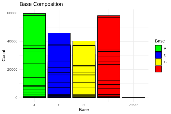
# Calculate base composition
base_composition <- alphabetFrequency(sequences, baseOnly = TRUE)
# Convert to data frame and reshape for ggplot2
base_composition_df <- as.data.frame(base_composition)
base_composition_df$ID <- rownames(base_composition_df)
base_composition_melted <- reshape2::melt(base_composition_df, id.vars = "ID", variable.name = "Base", value.name = "Count")
# Plot base composition bar chart using ggplot2
ggplot(base_composition_melted, aes(x = Base, y = Count, fill = Base)) +
geom_bar(stat = "identity", position = "dodge", color = "black") +
labs(title = "Base Composition",
x = "Base",
y = "Count") +
theme_minimal() +
scale_fill_manual(values = c("A" = "green", "C" = "blue", "G" = "yellow", "T" = "red"))
```
``` r
summary(sequence_lengths_df)
```
## Length
## Min. : 153
## 1st Qu.: 1162
## Median : 2850
## Mean : 5887
## 3rd Qu.: 6748
## Max. :199145
``` r
# Calculate base composition
base_composition <- alphabetFrequency(sequences, baseOnly = TRUE)
# Convert to data frame and reshape for ggplot2
base_composition_df <- as.data.frame(base_composition)
base_composition_df$ID <- rownames(base_composition_df)
base_composition_melted <- reshape2::melt(base_composition_df, id.vars = "ID", variable.name = "Base", value.name = "Count")
# Plot base composition bar chart using ggplot2
ggplot(base_composition_melted, aes(x = Base, y = Count, fill = Base)) +
geom_bar(stat = "identity", position = "dodge", color = "black") +
labs(title = "Base Composition",
x = "Base",
y = "Count") +
theme_minimal() +
scale_fill_manual(values = c("A" = "green", "C" = "blue", "G" = "yellow", "T" = "red"))
```
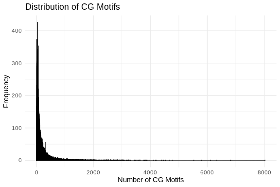
 ``` r
# Count CG motifs in each sequence
count_cg_motifs <- function(sequence) {
cg_motif <- "CG"
return(length(gregexpr(cg_motif, sequence, fixed = TRUE)[[1]]))
}
cg_motifs_counts <- sapply(sequences, count_cg_motifs)
# Create a data frame
cg_motifs_counts_df <- data.frame(CG_Count = cg_motifs_counts)
# Plot CG motifs distribution using ggplot2
ggplot(cg_motifs_counts_df, aes(x = CG_Count)) +
geom_histogram(binwidth = 1, color = "black", fill = "blue", alpha = 0.75) +
labs(title = "Distribution of CG Motifs",
x = "Number of CG Motifs",
y = "Frequency") +
theme_minimal()
```
``` r
# Count CG motifs in each sequence
count_cg_motifs <- function(sequence) {
cg_motif <- "CG"
return(length(gregexpr(cg_motif, sequence, fixed = TRUE)[[1]]))
}
cg_motifs_counts <- sapply(sequences, count_cg_motifs)
# Create a data frame
cg_motifs_counts_df <- data.frame(CG_Count = cg_motifs_counts)
# Plot CG motifs distribution using ggplot2
ggplot(cg_motifs_counts_df, aes(x = CG_Count)) +
geom_histogram(binwidth = 1, color = "black", fill = "blue", alpha = 0.75) +
labs(title = "Distribution of CG Motifs",
x = "Number of CG Motifs",
y = "Frequency") +
theme_minimal()
```
 ## 1.2 Database Creation
### 1.2.1 Obtain Fasta (UniProt/Swiss-Prot)
Already done during transcriptome annotation
`{r download-UniPSwissP-data, engine='bash'} cd ../../data curl -O https://ftp.uniprot.org/pub/databases/uniprot/current_release/knowledgebase/complete/uniprot_sprot.fasta.gz mv uniprot_sprot.fasta.gz uniprot_sprot_r2024_11.fasta.gz gunzip -k uniprot_sprot_r2024_11.fasta.gz`
### 1.2.2 Making the database
Already done during transcriptome annotation
`{r make-UniPSwissP-blastdb, engine='bash'} /home/shared/ncbi-blast-2.11.0+/bin/makeblastdb \ -in ../../data/uniprot_sprot_r2024_11.fasta \ -dbtype prot \ -out ../../data/blastdb/uniprot_sprot_r2024_11`
## 1.3 Running Blastx
``` bash
/home/shared/ncbi-blast-2.11.0+/bin/blastx \
-query ../data/02-Apul-reference-annotation/Apulcra-genome-mRNA.fa \
-db ../../data/blastdb/uniprot_sprot_r2024_11 \
-out ../output/02-Apul-reference-annotation/Apulcra-genome-mRNA-uniprot_blastx.tab \
-evalue 1E-20 \
-num_threads 40 \
-max_target_seqs 1 \
-outfmt 6
```
``` bash
echo "First few lines:"
head -2 ../output/02-Apul-reference-annotation/Apulcra-genome-mRNA-uniprot_blastx.tab
echo "Number of lines in output:"
wc -l ../output/02-Apul-reference-annotation/Apulcra-genome-mRNA-uniprot_blastx.tab
```
## First few lines:
## ntLink_4:1155-1537 sp|P35061|H2A_ACRFO 100.000 125 0 0 5 379 1 125 4.96e-86 249
## ntLink_4:2660-3441 sp|P84239|H3_URECA 99.265 136 1 0 371 778 1 136 5.03e-93 273
## Number of lines in output:
## 16190 ../output/02-Apul-reference-annotation/Apulcra-genome-mRNA-uniprot_blastx.tab
## 1.4 Joining Blast table with annoations.
### 1.4.1 Prepping Blast table for easy join
``` bash
tr '|' '\t' < ../output/02-Apul-reference-annotation/Apulcra-genome-mRNA-uniprot_blastx.tab \
> ../output/02-Apul-reference-annotation/Apulcra-genome-mRNA-uniprot_blastx_sep.tab
head -1 ../output/02-Apul-reference-annotation/Apulcra-genome-mRNA-uniprot_blastx_sep.tab
```
## ntLink_4:1155-1537 sp P35061 H2A_ACRFO 100.000 125 0 0 5 379 1 125 4.96e-86 249
### 1.4.2 Could do some cool stuff in R here reading in table
``` r
bltabl <- read.csv("../output/02-Apul-reference-annotation/Apulcra-genome-mRNA-uniprot_blastx_sep.tab", sep = '\t', header = FALSE)
spgo <- read.csv("https://gannet.fish.washington.edu/seashell/snaps/uniprot_table_r2023_01.tab", sep = '\t', header = TRUE)
datatable(head(bltabl), options = list(scrollX = TRUE, scrollY = "400px", scrollCollapse = TRUE, paging = FALSE))
```
``` r
datatable(head(spgo), options = list(scrollX = TRUE, scrollY = "400px", scrollCollapse = TRUE, paging = FALSE))
```
``` r
datatable(
left_join(bltabl, spgo, by = c("V3" = "Entry")) %>%
select(V1, V3, V13, Protein.names, Organism, Gene.Ontology..biological.process., Gene.Ontology.IDs)
# %>% mutate(V1 = str_replace_all(V1,pattern = "solid0078_20110412_FRAG_BC_WHITE_WHITE_F3_QV_SE_trimmed", replacement = "Ab"))
)
```
## 1.2 Database Creation
### 1.2.1 Obtain Fasta (UniProt/Swiss-Prot)
Already done during transcriptome annotation
`{r download-UniPSwissP-data, engine='bash'} cd ../../data curl -O https://ftp.uniprot.org/pub/databases/uniprot/current_release/knowledgebase/complete/uniprot_sprot.fasta.gz mv uniprot_sprot.fasta.gz uniprot_sprot_r2024_11.fasta.gz gunzip -k uniprot_sprot_r2024_11.fasta.gz`
### 1.2.2 Making the database
Already done during transcriptome annotation
`{r make-UniPSwissP-blastdb, engine='bash'} /home/shared/ncbi-blast-2.11.0+/bin/makeblastdb \ -in ../../data/uniprot_sprot_r2024_11.fasta \ -dbtype prot \ -out ../../data/blastdb/uniprot_sprot_r2024_11`
## 1.3 Running Blastx
``` bash
/home/shared/ncbi-blast-2.11.0+/bin/blastx \
-query ../data/02-Apul-reference-annotation/Apulcra-genome-mRNA.fa \
-db ../../data/blastdb/uniprot_sprot_r2024_11 \
-out ../output/02-Apul-reference-annotation/Apulcra-genome-mRNA-uniprot_blastx.tab \
-evalue 1E-20 \
-num_threads 40 \
-max_target_seqs 1 \
-outfmt 6
```
``` bash
echo "First few lines:"
head -2 ../output/02-Apul-reference-annotation/Apulcra-genome-mRNA-uniprot_blastx.tab
echo "Number of lines in output:"
wc -l ../output/02-Apul-reference-annotation/Apulcra-genome-mRNA-uniprot_blastx.tab
```
## First few lines:
## ntLink_4:1155-1537 sp|P35061|H2A_ACRFO 100.000 125 0 0 5 379 1 125 4.96e-86 249
## ntLink_4:2660-3441 sp|P84239|H3_URECA 99.265 136 1 0 371 778 1 136 5.03e-93 273
## Number of lines in output:
## 16190 ../output/02-Apul-reference-annotation/Apulcra-genome-mRNA-uniprot_blastx.tab
## 1.4 Joining Blast table with annoations.
### 1.4.1 Prepping Blast table for easy join
``` bash
tr '|' '\t' < ../output/02-Apul-reference-annotation/Apulcra-genome-mRNA-uniprot_blastx.tab \
> ../output/02-Apul-reference-annotation/Apulcra-genome-mRNA-uniprot_blastx_sep.tab
head -1 ../output/02-Apul-reference-annotation/Apulcra-genome-mRNA-uniprot_blastx_sep.tab
```
## ntLink_4:1155-1537 sp P35061 H2A_ACRFO 100.000 125 0 0 5 379 1 125 4.96e-86 249
### 1.4.2 Could do some cool stuff in R here reading in table
``` r
bltabl <- read.csv("../output/02-Apul-reference-annotation/Apulcra-genome-mRNA-uniprot_blastx_sep.tab", sep = '\t', header = FALSE)
spgo <- read.csv("https://gannet.fish.washington.edu/seashell/snaps/uniprot_table_r2023_01.tab", sep = '\t', header = TRUE)
datatable(head(bltabl), options = list(scrollX = TRUE, scrollY = "400px", scrollCollapse = TRUE, paging = FALSE))
```
``` r
datatable(head(spgo), options = list(scrollX = TRUE, scrollY = "400px", scrollCollapse = TRUE, paging = FALSE))
```
``` r
datatable(
left_join(bltabl, spgo, by = c("V3" = "Entry")) %>%
select(V1, V3, V13, Protein.names, Organism, Gene.Ontology..biological.process., Gene.Ontology.IDs)
# %>% mutate(V1 = str_replace_all(V1,pattern = "solid0078_20110412_FRAG_BC_WHITE_WHITE_F3_QV_SE_trimmed", replacement = "Ab"))
)
```