76 max transcript methylation

Lets take make a histogram of methylation for those genes that change methylation versus those that do not.. Need to grab one version of the files Sam made and joing with recent (40-based) methylation data

This only has transcripts that change.

female_tr <- read_csv("../output/34-transcript-counts/diffs.max.transcripts_per_gene.controls_females.vs.exposed_females.csv")

fmcoe_max_predom_isos <- read_csv("../supplemental-files/fmcoe-max-predom-isos.csv")

lets join

fmmax <- fmcoe_max_predom_isos %>%
  left_join(female_tr, by = "gene_name") %>%
  select(gene_name, control_females_max_transcript_counts.x, exposed_females_max_transcript_counts.x, difference)

lets join methylation data

female_40_meth <- read_csv("../output/73-gene-methylation/female_40_meth.csv") %>%
  mutate(name = str_replace(name, "gene-", ""))

structure(female_40_meth)

# A tibble: 38,523 × 3
   name         average_control average_exposed
   <chr>                  <dbl>           <dbl>
 1 ATP6                   1.22            1.49 
 2 COX1                   1.13            1.32 
 3 COX2                   1.20            1.36 
 4 COX3                   0.992           1.12 
 5 CYTB                   1.14            1.36 
 6 LOC111099029          52.9            57.3  
 7 LOC111099030           0.371           0.293
 8 LOC111099031           0.443           0.752
 9 LOC111099032           0.251           0.250
10 LOC111099033           0.380           0.311
# ℹ 38,513 more rows

col_name_1 <- names(fmmax)[1] # Get the name of the first column in fmmax
col_name_2 <- names(female_40_meth)[1] # Get the name of the first column in female_40_meth

# Perform the join
fmethmax <- left_join(female_40_meth,fmmax, by = setNames(col_name_1, col_name_2)) %>%
  mutate(mean_meth = (average_control + average_exposed)/2) %>%
  mutate(diff_meth = (average_exposed - average_control))

# Add a new column to indicate whether 'difference' is NA or not
fmethmax$diff_status <- ifelse(is.na(fmethmax$difference), "NA", "Not NA")

# Plot
ggplot(fmethmax, aes(x = mean_meth, fill = diff_status)) +
  geom_histogram(position = "identity", alpha = 0.5, binwidth = 1) + # Adjust binwidth as needed
  scale_fill_manual(values = c("NA" = "red", "Not NA" = "blue")) +
  labs(title = "Female gene methylation - change max transcript (not NA)",
       x = "Mean Methylation",
       fill = "Difference Status") +
  theme_minimal()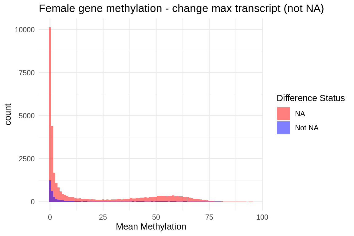

ggplot(fmethmax, aes(x = mean_meth)) + 
  geom_histogram(binwidth = 1, fill = "blue", color = "black") + # Adjust binwidth as needed
  facet_wrap(~diff_status, scales = "fixed") + 
  scale_y_log10() + # Apply log scale to y-axis) 
  labs(x = "Mean Meth", y = "Frequency") +
  theme_minimal() +
  ggtitle("Female gene methylation - change max transcript (not NA)")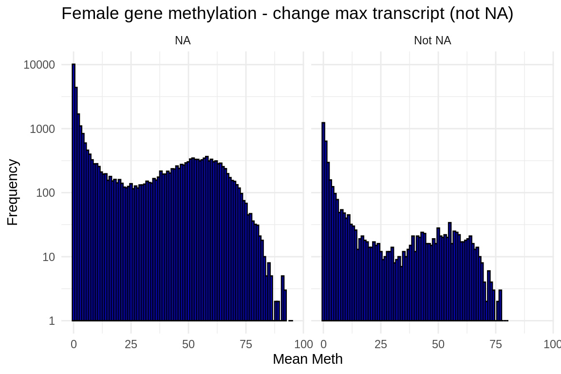

Plot

ggplot(fmethmax, aes(x = mean_meth, fill = diff_status)) + 
  geom_histogram(binwidth = 1) + # Adjust binwidth as needed
  scale_fill_manual(values = c("NA" = "red", "Not NA" = "blue")) +
  scale_y_log10() + # Apply log scale to y-axis) 
  labs(x = "Mean Meth", y = "Frequency") +
  theme_minimal() +
  ggtitle("Female gene methylation - change max transcript (not NA)")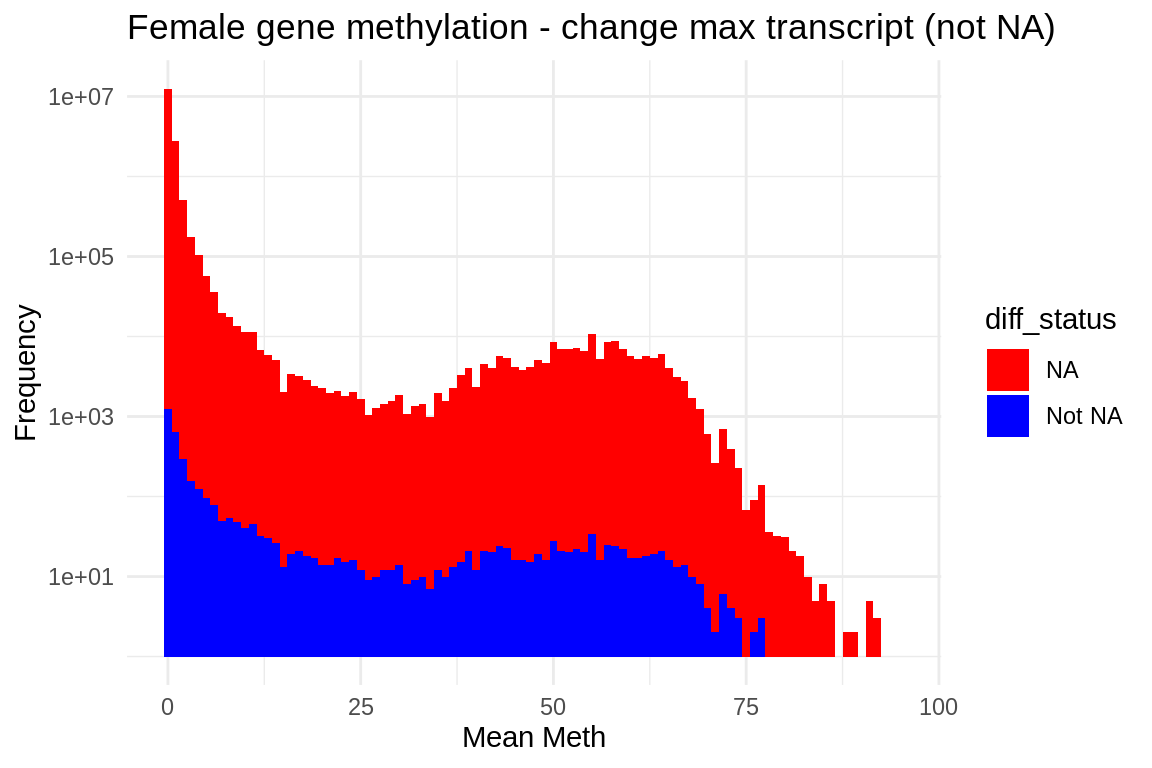

ggplot(fmethmax, aes(x = difference, y = diff_meth)) +
  geom_point() +  # This adds the points to the plot
  theme_minimal() +  # Optional: Applies a minimalistic theme
  labs(x = "Max transcript Difference", y = "Meth Difference", title = "max transcript vs. methylation") +
  geom_smooth(method = "lm", se = FALSE, color = "blue")  # Adds a linear regression line without confidence interval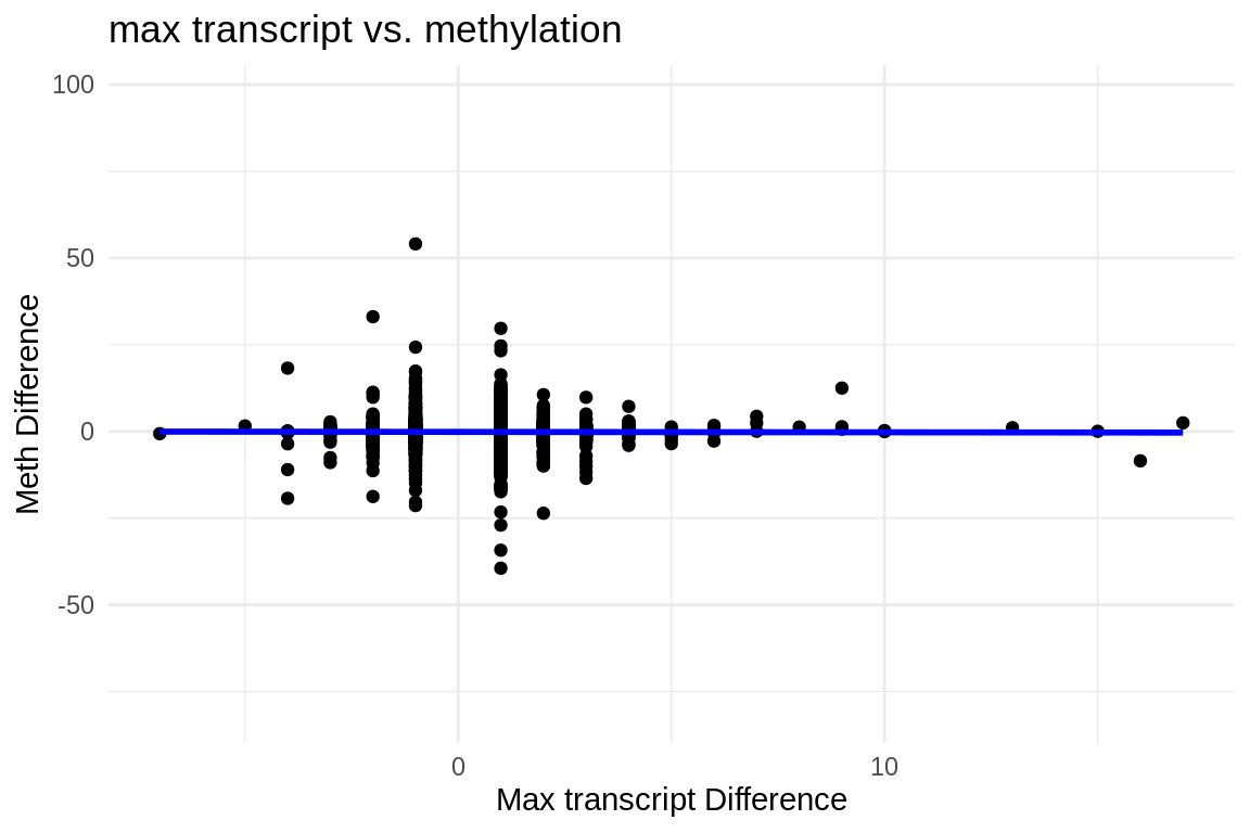

ggplot(fmethmax, aes(x = difference, y = diff_meth)) +
  geom_jitter() +  # This replaces geom_point() and adds jitter to the points
  theme_minimal() +  # Applies a minimalistic theme
  labs(x = "Max transcript Difference", y = "Meth Difference", title = "max transcript vs. methylation") +
  geom_smooth(method = "lm", se = FALSE, color = "blue")  # Adds a linear regression line without confidence interval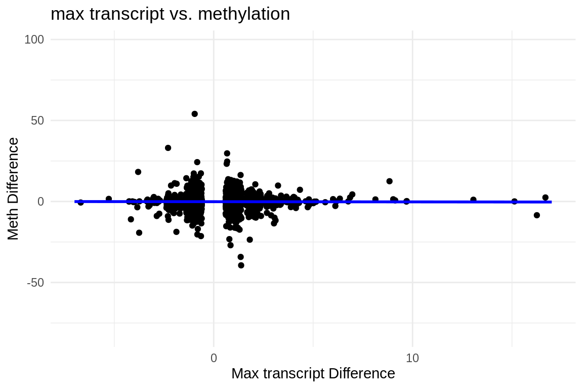

ggplot(fmethmax, aes(x = exposed_females_max_transcript_counts.x, y = average_exposed)) +
  geom_jitter() +  # This replaces geom_point() and adds jitter to the points
  theme_minimal() +  # Applies a minimalistic theme
  labs(x = "max transcript count", y = "gene methylation", title = "female exposed") +
  geom_smooth(method = "lm", se = FALSE, color = "blue")  # Adds a linear regression line without confidence interval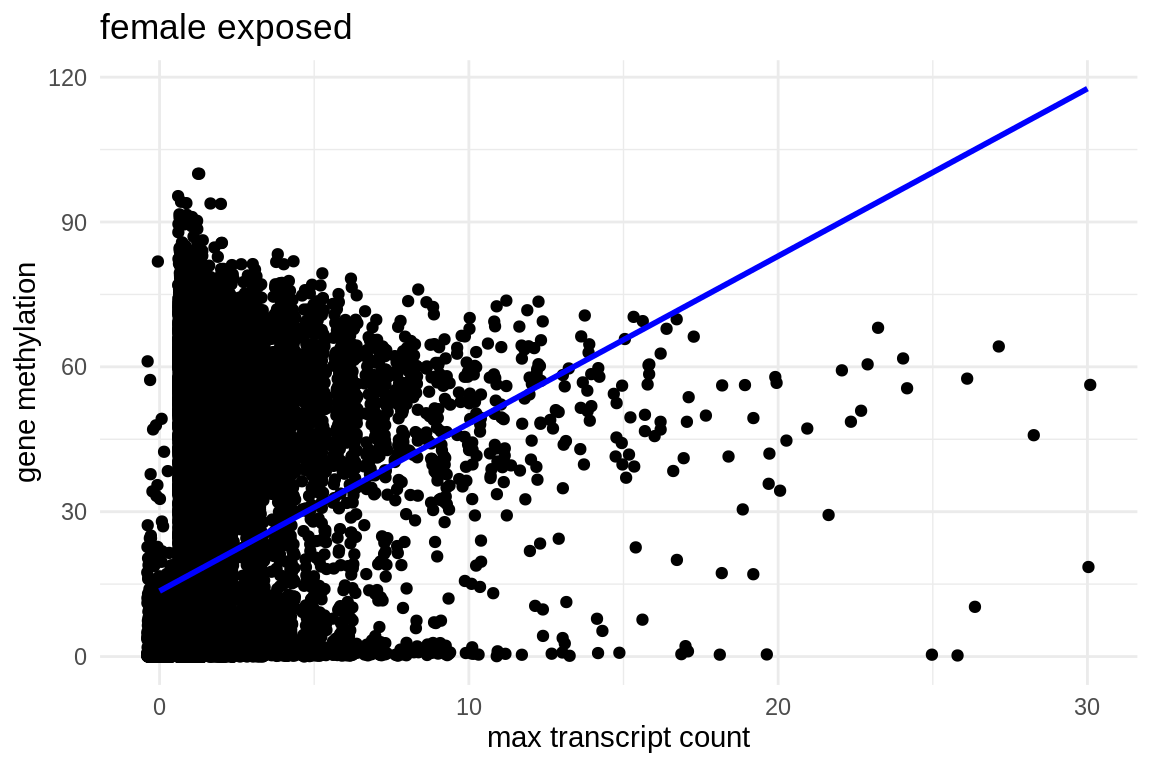

male

male_tr <- read_csv("../output/34-transcript-counts/diffs.max.transcripts_per_gene.controls_males.vs.exposed_males.csv")

mmax <- fmcoe_max_predom_isos %>%
  left_join(male_tr, by = "gene_name") %>%
  select(gene_name, control_males_max_transcript_counts.x, exposed_males_max_transcript_counts.x, difference)

lets join methylation data

male_40_meth <- read_csv("../output/73-gene-methylation/male_40_meth.csv") %>%
  mutate(name = str_replace(name, "gene-", ""))

col_name_1 <- names(mmax)[1] # Get the name of the first column in fmmax
col_name_2 <- names(male_40_meth)[1] # Get the name of the first column in female_40_meth

# Perform the join
mmethmax <- left_join(male_40_meth,mmax, by = setNames(col_name_1, col_name_2)) %>%
  mutate(mean_meth = (average_control + average_exposed)/2) %>%
  mutate(diff_meth = (average_exposed - average_control))

# Add a new column to indicate whether 'difference' is NA or not
mmethmax$diff_status <- ifelse(is.na(mmethmax$difference), "NA", "Not NA")

# Plot
ggplot(mmethmax, aes(x = mean_meth, fill = diff_status)) +
  geom_histogram(position = "identity", alpha = 0.5, binwidth = 1) + # Adjust binwidth as needed
  scale_fill_manual(values = c("NA" = "red", "Not NA" = "blue")) +
  labs(title = "Histogram of mean_meth",
       x = "Mean Methylation",
       fill = "Difference Status") +
  theme_minimal()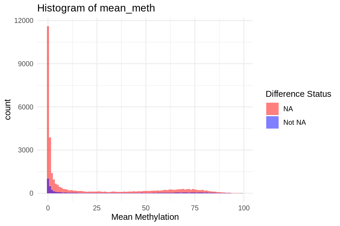

ggplot(mmethmax, aes(x = mean_meth, fill = diff_status)) + 
  geom_histogram(binwidth = 1) + # Adjust binwidth as needed
  scale_fill_manual(values = c("NA" = "red", "Not NA" = "blue")) +
  scale_y_log10() + # Apply log scale to y-axis) 
  labs(x = "Mean Meth", y = "Frequency") +
  theme_minimal() +
  ggtitle("Histogram of Mean Meth by Difference Status")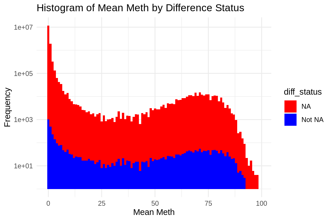

ggplot(mmethmax, aes(x = difference, y = diff_meth)) +
  geom_point() +  # This adds the points to the plot
  theme_minimal() +  # Optional: Applies a minimalistic theme
  labs(x = "Max transcript Difference", y = "Meth Difference", title = "max transcript vs. methylation") +
  geom_smooth(method = "lm", se = FALSE, color = "blue")  # Adds a linear regression line without confidence interval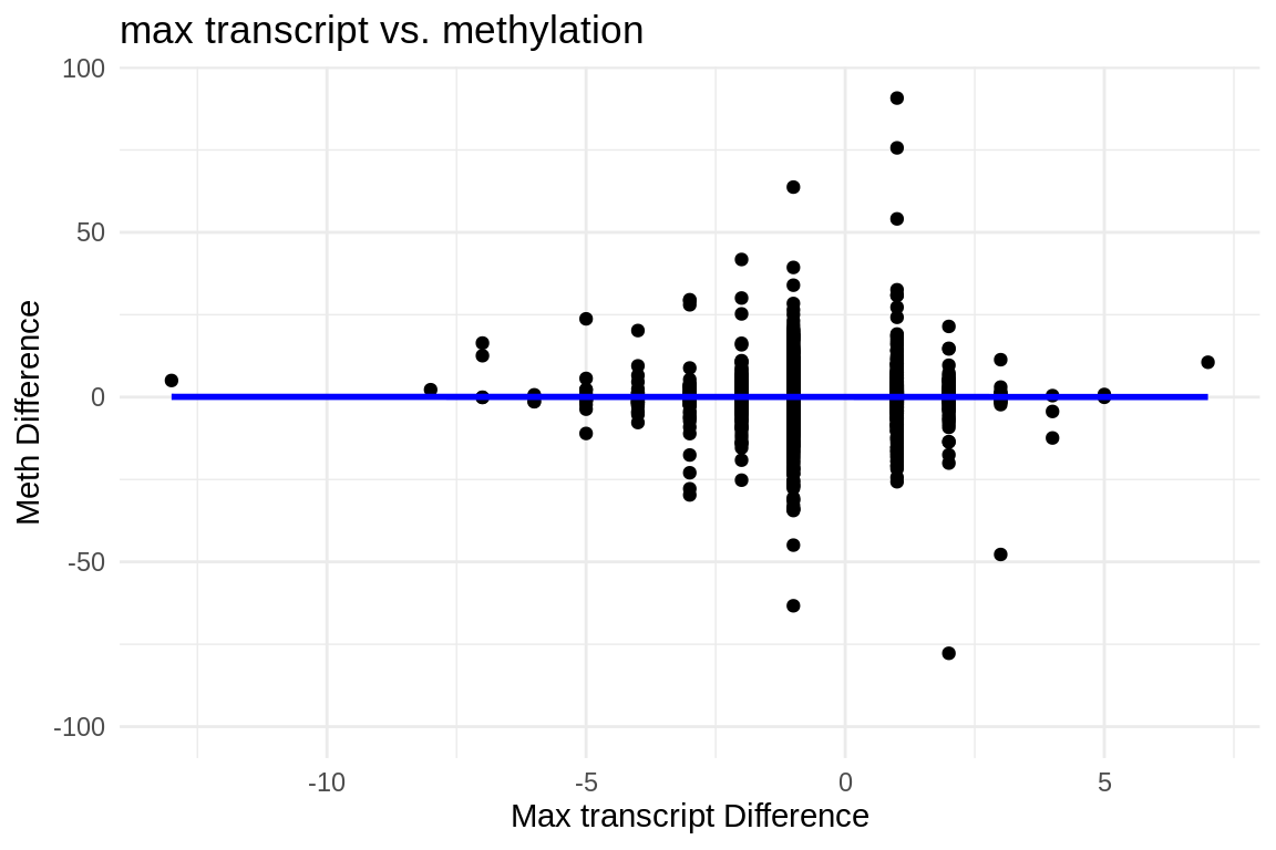

ggplot(mmethmax, aes(x = difference, y = diff_meth)) +
  geom_jitter() +  # This replaces geom_point() and adds jitter to the points
  theme_minimal() +  # Applies a minimalistic theme
  labs(x = "Max transcript Difference", y = "Meth Difference", title = "max transcript vs. methylation") +
  geom_smooth(method = "lm", se = FALSE, color = "blue")  # Adds a linear regression line without confidence interval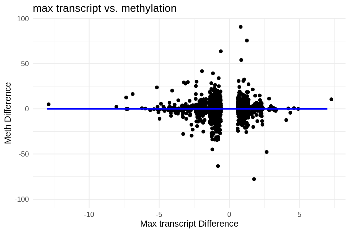

ggplot(mmethmax, aes(x = exposed_males_max_transcript_counts.x, y = average_exposed)) +
  geom_jitter() +  # This replaces geom_point() and adds jitter to the points
  theme_minimal() +  # Applies a minimalistic theme
  labs(x = "max transcript count", y = "gene methylation", title = "male exposed") +
  geom_smooth(method = "lm", se = FALSE, color = "blue")  # Adds a linear regression line without confidence interval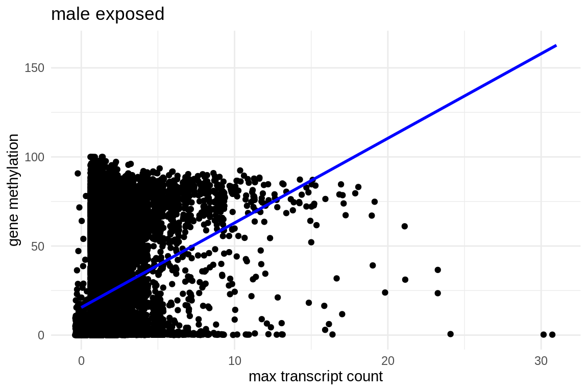

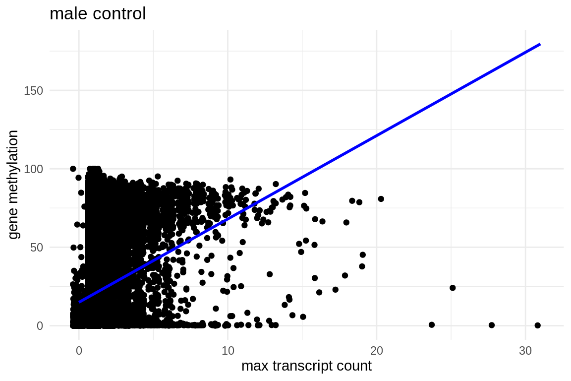
ggplot(mmethmax, aes(x = control_males_max_transcript_counts.x, y = average_control)) +
  geom_jitter() +  # This replaces geom_point() and adds jitter to the points
  theme_minimal() +  # Applies a minimalistic theme
  labs(x = "max transcript count", y = "gene methylation", title = "male control") +
  geom_smooth(method = "lm", se = FALSE, color = "blue")  # Adds a linear regression line without confidence interval