02-DGE-analysis
================
Kathleen Durkin
2025-04-08
- 1
Downloading reference
- 2 Downloading sequence reads
- 3 Running
DESeq2
Completing `Week 02` assignment of `FISH 546`, performing differential
gene analysis.
[Full assignment
details](https://sr320.github.io/course-fish546-2025/assignments/02-DGE.html)
# 1 Downloading reference
This code grabs the Pacific oyster fasta file of genes and does so
*ignoring* the fact that gannet does not have a security certificate to
authenticate (–insecure). This is usually not recommended however we
know the server.
``` bash
mkdir ../data/02-DGE-analysis
cd ../data/02-DGE-analysis
curl --insecure -O https://gannet.fish.washington.edu/seashell/bu-github/nb-2023/Cgigas/data/rna.fna
```
This code is indexing the file rna.fna while also renaming it as
cgigas_roslin_rna.index.
``` bash
/home/shared/kallisto/kallisto \
index -i \
../data/02-DGE-analysis/cgigas_roslin_rna.index \
../data/02-DGE-analysis/rna.fna
```
# 2 Downloading sequence reads
Sequence reads are on a public server at
This code uses recursive feature of wget (see this weeks’ reading) to
get all 24 files. Additionally, as with curl above we are ignoring the
fact there is not security certificate with –no-check-certificate
``` bash
cd ../data/02-DGE-analysis
wget --recursive --no-parent --no-directories \
--no-check-certificate \
--accept '*.fastq.gz' \
https://gannet.fish.washington.edu/seashell/bu-github/nb-2023/Cgigas/data/nopp/
```
The next chunk first creates a subdirectory
Then performs the following steps:
Uses the find utility to search for all files in the ../data/ directory
that match the pattern \*fastq.gz.
Uses the basename command to extract the base filename of each file
(i.e., the filename without the directory path), and removes the suffix
\_L001_R1_001.fastq.gz.
Runs the kallisto quant command on each input file, with the following
options:
-i ../data/cgigas_roslin_rna.index: Use the kallisto index file located
at ../data/cgigas_roslin_rna.index.
-o ../output/02-DGE-analysis/{}: Write the output files to a directory
called ../output/02-DGE-analysis/ with a subdirectory named after the
base filename of the input file (the {} is a placeholder for the base
filename).
-t 40: Use 40 threads for the computation.
–single -l 100 -s 10: Specify that the input file contains single-end
reads (–single), with an average read length of 100 (-l 100) and a
standard deviation of 10 (-s 10). The input file to process is specified
using the {} placeholder, which is replaced by the base filename from
the previous step.
``` bash
find ../data/02-DGE-analysis/*fastq.gz \
| xargs basename -s _L001_R1_001.fastq.gz | xargs -I{} /home/shared/kallisto/kallisto \
quant -i ../data/02-DGE-analysis/cgigas_roslin_rna.index \
-o ../output/02-DGE-analysis/{} \
-t 40 \
--single -l 100 -s 10 ../data/02-DGE-analysis/{}_L001_R1_001.fastq.gz
```
This command runs the abundance_estimates_to_matrix.pl script from the
Trinity RNA-seq assembly software package to create a gene expression
matrix from kallisto output files.
The specific options and arguments used in the command are as follows:
perl
/home/shared/trinityrnaseq-v2.12.0/util/abundance_estimates_to_matrix.pl:
Run the abundance_estimates_to_matrix.pl script from Trinity.
–est_method kallisto: Specify that the abundance estimates were
generated using kallisto.
–gene_trans_map none: Do not use a gene-to-transcript mapping file.
–out_prefix ../output/02-DGE-analysis: Use ../output/02-DGE-analysis as
the output directory and prefix for the gene expression matrix file.
–name_sample_by_basedir: Use the sample directory name (i.e., the final
directory in the input file paths) as the sample name in the output
matrix.
And then there are the kallisto abundance files to use as input for
creating the gene expression matrix.
``` bash
perl /home/shared/trinityrnaseq-v2.12.0/util/abundance_estimates_to_matrix.pl \
--est_method kallisto \
--gene_trans_map none \
--out_prefix ../output/02-DGE-analysis \
--name_sample_by_basedir \
../output/02-DGE-analysis/D54_S145/abundance.tsv \
../output/02-DGE-analysis/D56_S136/abundance.tsv \
../output/02-DGE-analysis/D58_S144/abundance.tsv \
../output/02-DGE-analysis/M45_S140/abundance.tsv \
../output/02-DGE-analysis/M48_S137/abundance.tsv \
../output/02-DGE-analysis/M89_S138/abundance.tsv \
../output/02-DGE-analysis/D55_S146/abundance.tsv \
../output/02-DGE-analysis/D57_S143/abundance.tsv \
../output/02-DGE-analysis/D59_S142/abundance.tsv \
../output/02-DGE-analysis/M46_S141/abundance.tsv \
../output/02-DGE-analysis/M49_S139/abundance.tsv \
../output/02-DGE-analysis/M90_S147/abundance.tsv \
../output/02-DGE-analysis/N48_S194/abundance.tsv \
../output/02-DGE-analysis/N50_S187/abundance.tsv \
../output/02-DGE-analysis/N52_S184/abundance.tsv \
../output/02-DGE-analysis/N54_S193/abundance.tsv \
../output/02-DGE-analysis/N56_S192/abundance.tsv \
../output/02-DGE-analysis/N58_S195/abundance.tsv \
../output/02-DGE-analysis/N49_S185/abundance.tsv \
../output/02-DGE-analysis/N51_S186/abundance.tsv \
../output/02-DGE-analysis/N53_S188/abundance.tsv \
../output/02-DGE-analysis/N55_S190/abundance.tsv \
../output/02-DGE-analysis/N57_S191/abundance.tsv \
../output/02-DGE-analysis/N59_S189/abundance.tsv
mv ../output/02-DGE-analysis.isoform* ../output/02-DGE-analysis/
```
# 3 Running DESeq2
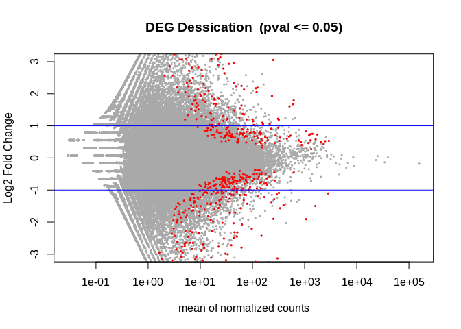
This code performs differential expression analysis to identify
differentially expressed genes (DEGs) between a control condition and a
desiccated condition.
First, it reads in a count matrix of isoform counts generated by
Kallisto, with row names set to the gene/transcript IDs and the first
column removed. It then rounds the counts to whole numbers.
Next, it creates a data.frame containing information about the
experimental conditions and sets row names to match the column names in
the count matrix. It uses this information to create a DESeqDataSet
object, which is then passed to the DESeq() function to fit a negative
binomial model and estimate dispersions. The results() function is used
to extract the results table, which is ordered by gene/transcript ID.
The code then prints the top few rows of the results table and
calculates the number of DEGs with an adjusted p-value less than or
equal to 0.05. It plots the log2 fold changes versus the mean normalized
counts for all genes, highlighting significant DEGs in red and adding
horizontal lines at 2-fold upregulation and downregulation. Finally, it
writes the list of significant DEGs to a file called “DEGlist.tab”.
Note The below code could be a single script (or single chunk). I like
separating to assist in troubleshooting and check output at various
steps.
Load packages:
``` r
library(DESeq2)
```
## Loading required package: S4Vectors
## Loading required package: stats4
## Loading required package: BiocGenerics
##
## Attaching package: 'BiocGenerics'
## The following objects are masked from 'package:stats':
##
## IQR, mad, sd, var, xtabs
## The following objects are masked from 'package:base':
##
## anyDuplicated, aperm, append, as.data.frame, basename, cbind,
## colnames, dirname, do.call, duplicated, eval, evalq, Filter, Find,
## get, grep, grepl, intersect, is.unsorted, lapply, Map, mapply,
## match, mget, order, paste, pmax, pmax.int, pmin, pmin.int,
## Position, rank, rbind, Reduce, rownames, sapply, setdiff, sort,
## table, tapply, union, unique, unsplit, which.max, which.min
##
## Attaching package: 'S4Vectors'
## The following objects are masked from 'package:base':
##
## expand.grid, I, unname
## Loading required package: IRanges
## Loading required package: GenomicRanges
## Loading required package: GenomeInfoDb
## Loading required package: SummarizedExperiment
## Loading required package: MatrixGenerics
## Loading required package: matrixStats
##
## Attaching package: 'MatrixGenerics'
## The following objects are masked from 'package:matrixStats':
##
## colAlls, colAnyNAs, colAnys, colAvgsPerRowSet, colCollapse,
## colCounts, colCummaxs, colCummins, colCumprods, colCumsums,
## colDiffs, colIQRDiffs, colIQRs, colLogSumExps, colMadDiffs,
## colMads, colMaxs, colMeans2, colMedians, colMins, colOrderStats,
## colProds, colQuantiles, colRanges, colRanks, colSdDiffs, colSds,
## colSums2, colTabulates, colVarDiffs, colVars, colWeightedMads,
## colWeightedMeans, colWeightedMedians, colWeightedSds,
## colWeightedVars, rowAlls, rowAnyNAs, rowAnys, rowAvgsPerColSet,
## rowCollapse, rowCounts, rowCummaxs, rowCummins, rowCumprods,
## rowCumsums, rowDiffs, rowIQRDiffs, rowIQRs, rowLogSumExps,
## rowMadDiffs, rowMads, rowMaxs, rowMeans2, rowMedians, rowMins,
## rowOrderStats, rowProds, rowQuantiles, rowRanges, rowRanks,
## rowSdDiffs, rowSds, rowSums2, rowTabulates, rowVarDiffs, rowVars,
## rowWeightedMads, rowWeightedMeans, rowWeightedMedians,
## rowWeightedSds, rowWeightedVars
## Loading required package: Biobase
## Welcome to Bioconductor
##
## Vignettes contain introductory material; view with
## 'browseVignettes()'. To cite Bioconductor, see
## 'citation("Biobase")', and for packages 'citation("pkgname")'.
##
## Attaching package: 'Biobase'
## The following object is masked from 'package:MatrixGenerics':
##
## rowMedians
## The following objects are masked from 'package:matrixStats':
##
## anyMissing, rowMedians
``` r
library(tidyverse)
```
## ── Attaching core tidyverse packages ──────────────────────── tidyverse 2.0.0 ──
## ✔ dplyr 1.1.4 ✔ readr 2.1.5
## ✔ forcats 1.0.0 ✔ stringr 1.5.1
## ✔ ggplot2 3.5.1 ✔ tibble 3.2.1
## ✔ lubridate 1.9.4 ✔ tidyr 1.3.1
## ✔ purrr 1.0.2
## ── Conflicts ────────────────────────────────────────── tidyverse_conflicts() ──
## ✖ lubridate::%within%() masks IRanges::%within%()
## ✖ dplyr::collapse() masks IRanges::collapse()
## ✖ dplyr::combine() masks Biobase::combine(), BiocGenerics::combine()
## ✖ dplyr::count() masks matrixStats::count()
## ✖ dplyr::desc() masks IRanges::desc()
## ✖ tidyr::expand() masks S4Vectors::expand()
## ✖ dplyr::filter() masks stats::filter()
## ✖ dplyr::first() masks S4Vectors::first()
## ✖ dplyr::lag() masks stats::lag()
## ✖ ggplot2::Position() masks BiocGenerics::Position(), base::Position()
## ✖ purrr::reduce() masks GenomicRanges::reduce(), IRanges::reduce()
## ✖ dplyr::rename() masks S4Vectors::rename()
## ✖ lubridate::second() masks S4Vectors::second()
## ✖ lubridate::second<-() masks S4Vectors::second<-()
## ✖ dplyr::slice() masks IRanges::slice()
## ℹ Use the conflicted package () to force all conflicts to become errors
``` r
library(pheatmap)
library(RColorBrewer)
library(data.table)
```
##
## Attaching package: 'data.table'
##
## The following objects are masked from 'package:lubridate':
##
## hour, isoweek, mday, minute, month, quarter, second, wday, week,
## yday, year
##
## The following objects are masked from 'package:dplyr':
##
## between, first, last
##
## The following object is masked from 'package:purrr':
##
## transpose
##
## The following object is masked from 'package:SummarizedExperiment':
##
## shift
##
## The following object is masked from 'package:GenomicRanges':
##
## shift
##
## The following object is masked from 'package:IRanges':
##
## shift
##
## The following objects are masked from 'package:S4Vectors':
##
## first, second
Might need to install first eg
``` r
if (!require("BiocManager", quietly = TRUE))
install.packages("BiocManager")
BiocManager::install("DESeq2")
```
Read in count matrix
``` r
countmatrix <- read.delim("../output/02-DGE-analysis/02-DGE-analysis.isoform.counts.matrix", header = TRUE, sep = '\t')
rownames(countmatrix) <- countmatrix$X
countmatrix <- countmatrix[,-1]
head(countmatrix)
```
## D54_S145 D56_S136 D58_S144 M45_S140 M48_S137 M89_S138 D55_S146
## XM_011449836.3 625.997 590.654 437.854 814.34600 551.397 529.09 497.03800
## XM_011422388.3 0.000 1.000 0.000 1.00000 2.000 1.00 0.00000
## XM_034446549.1 0.000 0.000 0.000 1.51743 0.000 0.00 1.51929
## XR_004596422.1 0.000 0.000 0.000 0.00000 0.000 0.00 3.00000
## XM_011441947.3 2.000 0.000 0.000 0.00000 0.000 0.00 0.00000
## XM_020063082.2 0.000 0.000 0.000 1.00000 1.000 1.00 0.00000
## D57_S143 D59_S142 M46_S141 M49_S139 M90_S147 N48_S194 N50_S187
## XM_011449836.3 808.653 597.057 820.993 849.273 694.19900 698.061 1046.56
## XM_011422388.3 0.000 1.000 2.000 0.000 0.00000 2.000 5.00
## XM_034446549.1 0.000 0.000 0.000 0.000 0.00000 0.000 0.00
## XR_004596422.1 0.000 1.000 0.000 0.000 0.00000 0.000 0.00
## XM_011441947.3 1.000 5.000 3.000 0.000 1.51259 0.000 1.00
## XM_020063082.2 0.000 0.000 0.000 0.000 0.00000 0.000 0.00
## N52_S184 N54_S193 N56_S192 N58_S195 N49_S185 N51_S186 N53_S188
## XM_011449836.3 725.657 695.765 42 912.862 742.214 953.086 867.709
## XM_011422388.3 2.000 0.000 0 1.000 1.000 0.000 1.000
## XM_034446549.1 0.000 0.000 0 0.000 0.000 0.000 0.000
## XR_004596422.1 0.000 0.000 0 0.000 0.000 0.000 0.000
## XM_011441947.3 1.000 0.000 0 0.000 1.000 2.000 1.000
## XM_020063082.2 0.000 0.000 0 0.000 0.000 0.000 1.000
## N55_S190 N57_S191 N59_S189
## XM_011449836.3 767.64 425.765 968.868
## XM_011422388.3 0.00 0.000 1.000
## XM_034446549.1 0.00 0.000 0.000
## XR_004596422.1 1.00 0.000 0.000
## XM_011441947.3 0.00 0.000 0.000
## XM_020063082.2 2.00 2.000 0.000
Round integers up to whole numbers for further analysis:
``` r
countmatrix <- round(countmatrix, 0)
str(countmatrix)
```
## 'data.frame': 73307 obs. of 24 variables:
## $ D54_S145: num 626 0 0 0 2 0 0 0 0 18 ...
## $ D56_S136: num 591 1 0 0 0 0 0 0 0 52 ...
## $ D58_S144: num 438 0 0 0 0 0 5 0 0 115 ...
## $ M45_S140: num 814 1 2 0 0 1 0 0 0 40 ...
## $ M48_S137: num 551 2 0 0 0 1 0 0 0 39 ...
## $ M89_S138: num 529 1 0 0 0 1 3 0 0 121 ...
## $ D55_S146: num 497 0 2 3 0 0 10 0 0 75 ...
## $ D57_S143: num 809 0 0 0 1 0 0 0 0 20 ...
## $ D59_S142: num 597 1 0 1 5 0 0 0 0 49 ...
## $ M46_S141: num 821 2 0 0 3 0 0 0 0 36 ...
## $ M49_S139: num 849 0 0 0 0 0 0 0 0 35 ...
## $ M90_S147: num 694 0 0 0 2 0 0 0 0 12 ...
## $ N48_S194: num 698 2 0 0 0 0 0 0 0 67 ...
## $ N50_S187: num 1047 5 0 0 1 ...
## $ N52_S184: num 726 2 0 0 1 0 0 0 0 209 ...
## $ N54_S193: num 696 0 0 0 0 0 0 0 0 37 ...
## $ N56_S192: num 42 0 0 0 0 0 0 1 0 5 ...
## $ N58_S195: num 913 1 0 0 0 0 0 0 0 13 ...
## $ N49_S185: num 742 1 0 0 1 0 6 0 0 73 ...
## $ N51_S186: num 953 0 0 0 2 0 0 0 0 8 ...
## $ N53_S188: num 868 1 0 0 1 1 0 0 0 32 ...
## $ N55_S190: num 768 0 0 1 0 2 0 0 0 13 ...
## $ N57_S191: num 426 0 0 0 0 2 0 0 0 95 ...
## $ N59_S189: num 969 1 0 0 0 0 0 51 0 34 ...
Get DEGs based on Desication
``` r
deseq2.colData <- data.frame(condition=factor(c(rep("control", 12), rep("desicated", 12))),
type=factor(rep("single-read", 24)))
rownames(deseq2.colData) <- colnames(data)
deseq2.dds <- DESeqDataSetFromMatrix(countData = countmatrix,
colData = deseq2.colData,
design = ~ condition)
```
## converting counts to integer mode
``` r
deseq2.dds <- DESeq(deseq2.dds)
```
## estimating size factors
## estimating dispersions
## gene-wise dispersion estimates
## mean-dispersion relationship
## final dispersion estimates
## fitting model and testing
## -- replacing outliers and refitting for 5677 genes
## -- DESeq argument 'minReplicatesForReplace' = 7
## -- original counts are preserved in counts(dds)
## estimating dispersions
## fitting model and testing
``` r
deseq2.res <- results(deseq2.dds)
deseq2.res <- deseq2.res[order(rownames(deseq2.res)), ]
```
``` r
head(deseq2.res)
```
## log2 fold change (MLE): condition desicated vs control
## Wald test p-value: condition desicated vs control
## DataFrame with 6 rows and 6 columns
## baseMean log2FoldChange lfcSE stat pvalue
##
## NM_001305288.1 0.181270 1.0453698 3.002647 0.348149 7.27728e-01
## NM_001305289.1 0.881457 -2.8119577 1.068276 -2.632239 8.48240e-03
## NM_001305290.1 145.913728 0.4580323 0.116185 3.942251 8.07203e-05
## NM_001305291.1 0.261701 0.5618449 1.587076 0.354013 7.23329e-01
## NM_001305292.1 2.902430 -1.2181330 0.763421 -1.595624 1.10573e-01
## NM_001305293.1 234.342117 0.0663449 0.131969 0.502731 6.15154e-01
## padj
##
## NM_001305288.1 NA
## NM_001305289.1 NA
## NM_001305290.1 0.00956401
## NM_001305291.1 NA
## NM_001305292.1 0.59541971
## NM_001305293.1 0.95562321
``` r
# Count number of hits with adjusted p-value less then 0.05
dim(deseq2.res[!is.na(deseq2.res$padj) & deseq2.res$padj <= 0.05, ])
```
## [1] 607 6
``` r
tmp <- deseq2.res
# The main plot
plot(tmp$baseMean, tmp$log2FoldChange, pch=20, cex=0.45, ylim=c(-3, 3), log="x", col="darkgray",
main="DEG Dessication (pval <= 0.05)",
xlab="mean of normalized counts",
ylab="Log2 Fold Change")
```
## Warning in xy.coords(x, y, xlabel, ylabel, log): 16484 x values <= 0 omitted
## from logarithmic plot
``` r
# Getting the significant points and plotting them again so they're a different color
tmp.sig <- deseq2.res[!is.na(deseq2.res$padj) & deseq2.res$padj <= 0.05, ]
points(tmp.sig$baseMean, tmp.sig$log2FoldChange, pch=20, cex=0.45, col="red")
# 2 FC lines
abline(h=c(-1,1), col="blue")
```
``` r
write.table(tmp.sig, "../output/02-DGE-analysis/DEGlist.tab", row.names = T)
```